Phastware © 2017 Phastware Consulting
Phastline Application Documentation
General Overview
Phastline is a batched pipeline simulation program and is now available for use free of charge. Please review the information below and if interested in using the application, use the "Sign-Up" link provided to register an account and begin using the application right away. If you have any questions or need support on how to use the application you may get in touch with the developer at wmshockey@gmail.com. Thank-you.
Phastline simulates the operation of a batched or single product liquid pipeline. By providing the application with a physical description of the pipeline such as length, diameter, elevation, station location, pumps etc. and the type of product to be shipped, the application will calculate and report the hydraulic gradients, pressures, flowrates, power and energy. It takes the products to be shipped in the form of a nomination, breaks the volumes into batches and simulates the movement of those batches through the pipeline, taking into account intermediate injections and deliveries at stations along the line. Batch injections will be scheduled out over the course of the simulation to evenly spread the volumes provided by each shipper.
The maximum flowrate or capacity of the pipeline will be determined and the pressure profile at each step in time during the simulation will be calculated. Pump curves will be combined at the stations to determine the discharge pressures and the Colebrook-White formula for line loss will be used to calculate the pressure losses between stations. At no point will pressures exceed the maximum allowed pressure of the pipe or go below the vapour pressures of the fluids in the line. Viscosity and density of the fluids will be corrected for temperature. A report is provided that shows where the bottlenecks are located on the pipeline which are the points limiting the rate of flow.
Users can modify the physical attributes of the pipeline to determine the effect of each change on pressures, flow rates and power/energy consumption.
Technical Requirements
Phastline is an entirely web-based application and only requires an internet browser on the users PC or laptop. The compatible browsers on Windows 10 are MS Edge, Google Chrome and Mozilla Firefox. Internet Explorer does NOT work. Compatible browsers on Mac OSX are Safari, Google Chrome and Mozilla Firefox. The application will also run in iOS on Apple iPads or iPhones and Android smartphones and tablets.
Input Data Requirements
The application needs to know specifics of the pipeline and products to be shipped through it before it can run a simulation of its operation. The diagram below shows an overall structure of the data used by the application.
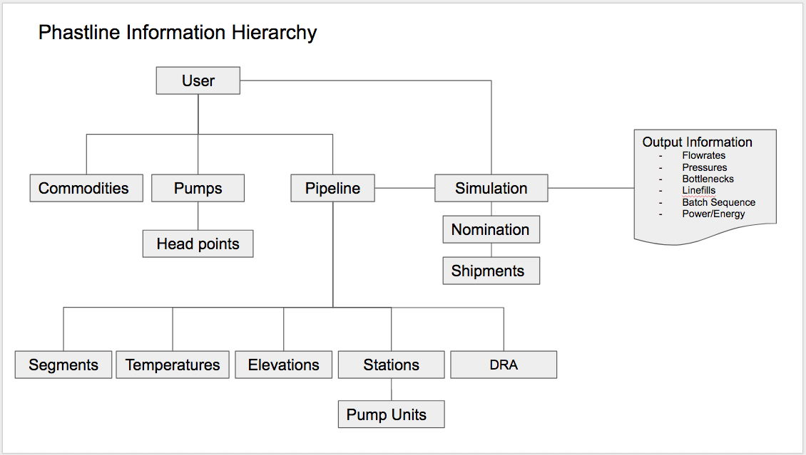
Users
When a person signs-up to use the application, they become an authorized user and can begin to use the application. A new user will be provided with an initial set of seed data consisting of two sample pipelines and a set of pump characteristics and commodity characteristics as examples of how to set up the input data. The user can then run simulations on these two sample pipelines or begin to create their own pipelines and simulations. A user owns each pump, commodity, pipeline and simulation that they create. Each user's data is completely separate and no two users can see each other's data.
Commodities
Commodities are the products that are shipped through the pipeline. Each commodity will have an ID which is an abbreviation that is unique and that will be used to identify the batches in the pipeline. Also, each commodity needs to have its fluid properties recorded, which consists of:
- Commodity ID
- viscosity at two different temperatures
- Density at one temperature and a density correction factor to calculate what its density will be at other temperatures
- Vapour pressure of the fluid
Pumps
Pumps are identified by a pump ID (e.g. B-C-517). Each pump has a head curve which is a series of (flowrate, head) data points. "Head" is the unit commonly used to measure the pressure output of a pump and refers to the height that a column of fluid would rise to if coming straight out the discharge side of the pump. The head or pressure, generated by a pump typically decreases as the rate of flow increases.
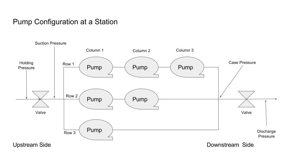
Pump Units
Pumps are installed at stations in series or parallel combinations. Each pump is placed in a certain row and column position. Pumps on the same row are in series whereas pumps in parallel on on different rows. The flowrate through a station is divided up equally across each row of the pump configuration. For pumps in series, the discharge side of one pump is fed into the suction side of the pump in the next column position. Pumps are considered incompatible if the heads that they generate do not overlap over some range of flowrates.
Pipeline Segments
Pipeline segments are sections of pipe that have the same physical properties, specifically:- Diameter
- Wall Thickness
- Roughness
- Maximum Allowable Working Pressure (MAWP)
The roughness of a pipe refers to how smooth the inside wall of the pipe is and is measured in meters or inches so is an extremely small fractional number. Obviously, the rougher the pipe, the more line loss there is along the pipe. Typically the wider the wall thickness, the higher the MAWP. Pipe segments are connected in series and their position in the line shown as the kilometer post at which the pipe segment starts. The diameter of the pipe is the single most important factor in determining the flowing pressure loss in the pipe. According to the Colebrook-White line loss formula, the pressure loss varies as the 5th power of the diameter.
Pipeline Stations
Stations are the points along the pipeline where pumping units are installed and can also be locations where injections or deliveries can occur. The location of a station along the line is designated by a kilometer post.
Pipeline Elevations
A pipeline has an elevation profile as it follows the contour of the land over which it is constructed. An elevation profile is a series of (kmp, elevation) data points. The elevation profile is important since there are static pressure losses and gains along the pipeline that effect the hydraulics of the line. As the pipeline goes uphill, pressure is lost and conversely as it goes downhill, pressure is gained. The gain or loss in pressure also depends on the density of the product in the line.
Pipeline Temperatures
An estimated pipeline temperature profile is required so that the program can calculate the changes to both viscosity and density of the product in the line. For higher temperatures, the viscosity of a fluid typically decreases resulting in lower pressure loss as it is pumped through the line. Similarly for density, a fluid has slightly lower density at a higher temperatures. The temperature profile is a series of data points with (kmp, temperature) values.
Drag Reducing Agents
Drag Reducing Agents (DRA) or "flow improvers" can be specified for various sections of the pipeline. DRA is an chemical additive injected into the pipeline to reduce turbulence in the pipe and reduces the amount of pressure loss down the pipeline. A percentage reduction in pressure loss may be specified over a certain range of the pipeline to model the effect on the line. For example, a DRA value of 70 would reduce the amount of pressure loss due to flow turbulence over the distance range specified by 70%, thus resulting in increased pipeline flowrate capacity and/or less power consumption to run the line. Typical values for various commercial flow improvers range from 20% to 80%.
Nominations
A nomination is what a pipeline company typically receives from its shipper customers on a monthly basis. A nomination consist of the type of commodity the shipper wishes to move through the pipeline, a volume and the starting (receipt) and ending (delivery) locations over which the product will travel. When nominations are received, the program will break the volumes up into smaller batches according to a user specified maximum batch size. The program will then sequence the batches in the order in which they will be pumped over the month in a manner that evenly distributes the batch injections over that time period. This is so that no one shipper is over taxed to provide all of its nominated volume all at once to the pipeline. Shipper's have supply and feeder pipeline facilities with limited capacity and this has to be taken into account. A nomination typically corresponds to one calendar month pumping period and will consist of multiple shipments of different commodities from multiple shippers. Each of the desired shipments is usually of a volume higher than what can be practically shipped down the line in one batch. A nomination consists of shipments where each shipment will have the following data values:
- Start (Receipt) station
- End (Delivery) station
- Commodity type
- Volume
- Shipper
Calculations and Processing
Line pipe Modeling:
The program performs the following calculations to model pipe segments:
- Line pressure loss accounting for variations in elevation, pipe diameter, roughness and fluid viscosity and density.
- Viscosity and density changes computed using exact batch positions.
- Implicit form of Colebrook White friction factor formula.
- Darcy Weisbach flowing pressure loss formula.
- Line pressure is constrained to be below specified maximum allowable operating pressure at all points. Excess pressure is throttled.
- Line pressure is set to vapour pressure at full stream injection points.
Station Modeling:
Stations are modeled as follows. Note that not all stations have pumps and not all stations will have injection or delivery operations occurring at them.
- Series and parallel pump configurations may be specified
- Pump pressure is interpolated directly from the flow/head points specified in the pump characteristics table.
- An overall station curve is constructed that will yield the maximum pressure available at the station with all pump units turned on
- Injection or Receipt activities are simulated by shutting down the line upstream and allowing the new batch to enter the line at the station.
- Landing or Delivery activities are simulated by shutting down the line downstream and allowing the batch to leave the line at the station.
Pump Curve Combinations
Station curves are calculated by adding the pressures of all pumps on the same row at common flow rate values. If there is more than one row of pumps at a station (parallel operation) the flow rates of each row are added at common pressure values.
Pump Head Calculation
The pressure gain created through the action of a pump in the line is simply modeled from flow vs pressure curves supplied from the Pump Characteristics file. Normally, the higher in flowrate, the less pressure a pump can generate. These curves are in the form of several points (e.g. 15). Pumps are identified by a unique 10 character pump name. Each pump may have several curves, one for each different range of viscosity. The performance of a pump is dependent on the viscosity of the fluid being pumped. The density of the fluid in the pump also has a significant effect on the pressure generated but it does not change the shape of the performance curve as viscosity does.
The following formula is used for computing the pressure generated by a pump:
pres = (gcons/1000) * dens * head
where:
pres = pressure gain through a pump (kpa)
gcons = acceleration due to gravity (9.806 m/sec**2)
/1000 = conversion from pascals to kilopascals (kpa)
dens = density of fluid in pump (kg/m3)
head = meters of head of water interpolated from curve
Line Loss Formula
Lineloss is the total pressure lost (or gained) along the pipe from one station to the next. There are two components to lineloss (static and dynamic). Static lineloss is the pressure variation along the line caused by elevation differences (i.e pressure is lost going uphill and gained coming downhill). Denser batches lose more pressure going uphill than lighter batches.
Static Lineloss formula: PS = G * dens * elevwhere:
- PS = Static pressure loss (or gain) in kpa
- G = Acceleration due to gravity (9.80652)
- dens = Density (kg/m3)
- elev = Elevation difference (meters)
Dynamic Lineloss: Dynamic (or flowing) pressure loss refers to pressure lost along the line due to the internal friction of the fluid against the inside pipe wall. This pressure is lost in the form of heat. The calculation is actually a three step procedure:
- Compute Reynolds number
- Compute Friction Factor
- Compute Lineloss
Reynolds number formula:
reynl = kreyn * flow/(diam*visc)
where:
reynl = Reynolds number kreyn = Constant (353.677499) flow = flowrate (m3/hr) diam = diameter (meters) visc = viscosity (centistokes)Friction Factor calculation:
if reynl > 40000 then use Colebrook-White formula:
frict= SQRT(1/(-2*LOG( ruff/(diam*3700) + 5.74/(reynl**0.9)) ))
if 2500 < reynl < 40000 then:
frict = 0.364 / (reynl**0.265)
if 2000 < reynl < 2500 then:
frict = (reynl**1.596) / 5700000
if 0 < reynl < 2000 then:
frict = 64/reynl
where:
frict = friction factor
reynl = Reynolds number
ruff = roughness of pipe (millimeters)
diam = diameter (meters)
SQRT = notation to mean "square root of"
LOG = base 10 logarithm
** = notation to mean "to the power of"
Dynamic Lineloss formula (Darcy-Weisbach):
loss = kdarc * dens * frict * (flow**2) / (diam**5)
where:
kdarc = constant (6.254)
dens = density (kg/m3)
frict = friction factor
flow = flowrate (m3/hr)
diam = diameter (meters)
loss = pressure loss (kpa/kilometre)
Viscosity and Density Fluid Properties
The two fluid properties modelled by this program are viscosity and density. Both of these properties are functions of temperature.
Viscosity:
The viscosity attributes for each fluid id contained in the fluid properties file consist of two viscosity/temperature points (V1,T1) and (V2,T2). The ASTM method is used to compute the viscosity V at some temperature T given V1,T1 and V2,T2. Using the two viscosity points read in from the file the program solves the following equation to get two coefficients for each fluid (A and B):
LOG(LOG(Z)) = A - B*LOG(T)where:
Z = V + 0.7 + EXP( -1.47 - 1.84*V - 0.51*(V*V) )
V = kinematic viscosity in centistokes (mm**2/sec)
T = Temperature in degrees kelvin
A = first viscosity coefficient
B = second viscosity coefficient
LOG = Base 10 logarithm
Using the same formula, the program adjusts viscosities along the line to the temperatures specified at that point.
Density:
The density attributes for each commodity contained in the commodity table consist of a density at 15 degrees C and a density correction factor. The program then uses the following formula to adjust the specified 15 deg C density to line temperatures:
D = D15 * DCF**(T-15)where:
D = Density at temperature T
D15 = Density at 15 degrees C
DCF = Density correction factor
T = Temperature at a point on the line
** = notation to mean "raised to the power"
Power Calculation:
The power shown in the application's reports is hydraulic power imparted to the fluid and is expressed in Kilowatts. The formula used is:
Power = Q * dP / 3600
where:
- Q = Flowrate in m3/hr
- dP = differential pressure across the pumps in Kpa
Capacity Flowrate Calculation
The "Capacity" flowrate is computed using successive iterations until the line pressure is within 1 kpa of vapour pressure at some point on the line. The minimum difference between line pressure and vapour pressure is termed the "violation amount".
Successive flowrate values are computed using linear interpolation based on the previous two flowrates and violation amounts. Note that a negative violation amount means there is no violation and the negative value is a measure of how much room there is until a violation is reached (over MAWP or under vapour pressure).
Batch Sizing and Sequencing
The volumes of product desired to be shipped on the line are specified in the nomination. These volumes are typically broken up into smaller standard size batches so that a shipper is not required to supply all of it at one time. The standard size of the batches is set by the user when they run a simulation (e.g. 10,000 m3). Once the shipments are broken up into batches, they are sequenced in an order that ensures equitable distribution of injections from each shipper over the course of the simulation period (typically one month).
Bottleneck Calculation
The bottleneck percentages listed in the summary results display following a simulation show the percentage of times each station is considered to be a "bottleneck". When a station is tagged as being a bottleneck, that means that at some point in the line between it and the next station, there is a low pressure point that is close to the vapour pressure of the fluid in the line at that point in time. If the intention is to increase the capacity of a pipeline, those stations that show high bottleneck percentages should be given consideration for either adding additional pumps or replacing line segments downstream of the station with wider diameter pipe or higher MAWP ratings.
Initial Linefill
The batches in the line at the start of the simulation are set so that the last batch of the batch sequence lies fully downstream of the first station in the line. This way, the first batch to be injected at the first station will be the first batch of the bactch sequence.
How to Use the Application
The Phastline application is intended to be a training tool for someone interested in understanding how a batched liquid pipeline is designed and operated. As a design tool, the user can evaluate different variations of pipe diameter, size, station spacing and pump installations to see how each change effects the overall pipeline capacity. As an operational tool, the user can configure pipeline as it currently exists, then use current or forecasted nomination volumes to run through it to determine the power and energy usage which could ultimately determine the cost of operating the pipeline.
The user is provided with sample set of data when they first sign-up to use the application. This includes:
- Commodity properties for about 24 different commodities
- Pump data for about 12 different pumps
- Pipeline data for two different pipelines. One example is for an actual pipeline operated by a large North American pipeline company. The other is a simple fictional 3 station line with only a few nominated shipments.
For running their own studies, a user would typically start out by setting up the input data for the pipeline they are interested in as follows.
- Create a Pipeline. Enter the data points for where the stations are located on the line, where the segments are, what the elevations are and what temperatures are.
- Create a Nomination and enter the shipments desired to be pumped through the line.
- Run a Simulation. With the Pipeline and Nomination data finalized, the user would then run a new simulation. Running a new simulation is simply a matter of giving it a name and then specifying the Pipeline and Nomination to be used.
- The Maximum Flowrate is a constraint that is imposed on the simulation to make sure that at no point in time will the flowrate go higher than the value specified at any point on the line. This value can be set to an arbitrarily high value so that the program will calculate and use the capacity flow rate for the line.
- The Maximum Batch size is used to break up the nominated shipments into batches.
- The Maximum Step Time is the upper limit to how long the duration of a time step is in performing the simulation. Shorter a Max Step Time will mean greater precision in the hydraulic gradients but will take longer running time on the computer to complete the simulation.
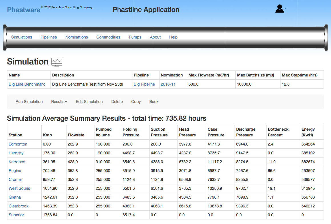
- Average Summary Results
- Batch Sequence - an overall summary of the entire pipeline schedule
- Power/Energy - report showing the total power and energy consumption of the pipeline
- Station Curves - shows the combined flowrate/pressure curve for each station
- Station Detail - Flowrate, pressure and power at a station over the course of the simulation
- Station Step Detail - Flowrate, pressure and power at a station shown step by step
- Step Detail - Flowrate, pressure and power for the pipeline shown step by step
- Step Flowrates - Flowrates across the line shown step by step
- Step Linefill - The linefill (batch positions) shown step by step
Running a Simulation
Running a simulation is simply a matter of selecting it form the index list of simulations shown on the first screen in the application, then pressing the "Run Simulation" button. The length of time the program takes to complete the simulation depends on how large the pipeline is (pipeline length and number of stations) and how large the nominated shipments are (large volumes mean large number of batches). Simulations typically take from a few seconds to a minute, depending on how large the pipeline is and how many batches there are.
Viewing Output displays and reports
When a simulation completes successfully, a menu will be shown on screen that allows the user to view the output results from a number of different perspectives. He/she can look at the average summary results, the linefills at each step, the pressures at each station in each step, the total power and energy consumed.The current list of display available for viewing the simulation results are:
Sample Display
Sign In and Sign out of User Accounts
A user would typically start out by going to the www.phastware.com website and reading about the Phastline application by selecting the "documentation" link. If interested, you can contact me at wmshockey@gmail.com and I will create an account for you with a username and initial password. The new account will have a set of initial data seeded for it including sample pipeline, nomination, pump and commodity data. Now the user can sign-in to their account and start creating/modifying pipelines and running simulations.
Technical
Phastline is an entirely web-based application. It does not require anything to be installed on the user's PC or laptop. All data is stored in a back-end SQL database and all front-end screens and processing were coded using the Ruby on Rails application development environment with the MVC (Model-View_Controller) architecture. All data in a users's account is secured in the SQL database and separate from other user's data. If a user prefers the application to be installed directly on a PC or laptop, then that is also an option but will require some work on my part to install the necessary software on your machine.
Future Enhancements
The application is under continuous development and refinement so version upgrades are frequent. All enhancements and bugs are being recorded in a JIRA project database. The first release of the application (version 1.1) was in December 2017. If you are interested in being notified about what future enhancements are planned or have suggestions yourself, please contact Warren Shockey by email at wmshockey@gmail.com.